Kate Robertson1, 2, Stephan Thiel1, 2 and Naser Meqbel3, 4
1 Geological Survey of South Australia, Department for Energy and Mining
2 School of Physical Sciences, University of Adelaide
3 The Helmholtz Centre Potsdam-GFZ German Research Centre for Geosciences
4 Currently at National Observatory of Brazil
Download this article as a PDF (7.2 MB); cite as MESA Journal 92, pages 12–18
Published April 2020
Introduction
South Australia has some of the highest magnetotelluric (MT) station coverage worldwide providing a unique opportunity to understand lithospheric architecture of the state and ultimately reduce the exploration risk for mineral occurrences. Over the last 15 years there have been a number of 2D MT profiles across the state to investigate its tectonic evolution (Thiel, Heinson and White 2005; Selway et al. 2011; Thiel and Heinson 2010), explore its mineral potential (Thiel et al. 2016; Heinson et al. 2018) and to integrate with other datasets (Wise and Thiel 2019). While 2D modelling of profile data has become standard, many areas are prone to 3D effects and are inadequately modelled using a 2D approach. As a result, data collected in a semi-regular array and modelled in 3D has become more common (Robertson, Heinson and Thiel 2016; Thiel and Heinson 2013).
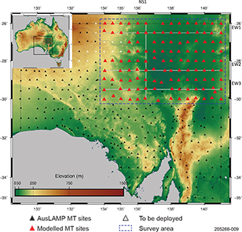
Figure 1 Topography map showing AusLAMP sites and the location of transects EW1, EW2, EW3 and NS1 shown in later figures. Reprinted from Robertson, Thiel and Meqbel (2020, fig. 1 with locality map inset) under Creative Commons Licence CC BY 4.0.
The flagship Australian Lithospheric Architecture Magnetotelluric Project (AusLAMP) SA program collected ~400 long-period MT stations every half degree latitude and longitude across South Australia between 2014 and 2018 (Fig. 1). More recently, the Olympic Domain ultra-wide band MT survey across the eastern Gawler Craton margin was undertaken as an infill of AusLAMP sites and is an array of sites exceeding 300 stations across an area of 100 x 100 km. Robust resistivity models of these arrays necessitate the use of new 3D inverse modelling codes, which are now computationally feasible to run with supercomputing facilities, such as the National Computational Infrastructure in Canberra. To realise the benefits of these new datasets, it is essential to test robustness of the resistivity models thus produced.
With the increased complexity of 3D modelling comes opportunities for the models to be influenced by a wider set of variables, potentially leading to modelling artefacts. To develop best practice for our 3D modelling approach, we have undertaken a significant study to test robustness of our modelling. This article presents a summary of our study, recently published in the open access journal Earth, Planets and Space (Robertson, Thiel and Meqbel 2020) and provides insights into testing various modelling parameters. We applied parameterisation tests to a 3D MT inversion of the AusLAMP dataset in the northeastern part of South Australia.
Magnetotelluric inversion
The geophysical inversion of MT data is a non-unique inverse problem, meaning that there are many solutions or models that fit the data equally well. For this reason, it is critical to understand the range of models that can fit the data, ie to explore the model space and ensure the features in the presented model are robust. This is especially the case if only one model is presented; ideally the whole ensemble of models that can fit the data (preferably within petrological constraints) would be provided with an associated uncertainty, which is commonplace in 1D, available but not readily used in 2D, and becoming possible in 3D with the advance in supercomputing performance and inversion code development. The earth is three-dimensional, but sometimes approximates to 1D (sedimentary basins) or 2D. The complexity of the inverse problem increases greatly as we move from 1D, to 2D then 3D inversion, and thus it is much more common to present in 3D a geophysical model that is not as robust or as well-tested as its 1D or 2D counterpart.
The purpose of our investigation was to understand the effects of changes in inversion parameters on the final model, the significance of incorporating different components of the data, and the inclusion of prior information in the inversion (biasing the model). The investigations were undertaken using the open-to-academia 3D inversion code, ModEM3DMT (Egbert and Kelbert 2012; Kelbert et al. 2014) on the Raijin supercomputer of the National Computational Infrastructure (supported by the National Computational Merit Allocation Scheme). A subset of 123 AusLAMP long-period MT sites from the northeast of South Australia was inverted for a variety of parameters that pertain to the geology and the data across the study area, as well as inversion modelling parameters. For the inversion parameters, we tested different model covariances (higher covariance results in smoother models), lambda values (a trade-off parameter between data fit and model smoothness), and the cell size of the model. Various representations of the geology and data include testing differences in electrical resistivities of starting models, and different levels of assumed prior information about the resistivity of the subsurface (eg bathymetry, sediments, phase transitions of mantle minerals and associated changes in resistivity), and the components of the data that were inverted for (MT or geomagnetic transfer functions). Some of the more important outcomes are summarised here, but the reader is encouraged to see Robertson, Thiel and Meqbel (2020) for more detail.
Results and discussion
Inclusion of known information into starting models
Inversion codes require the input of a starting model, from which the inversion code moves away from and toward a solution to the inverse problem. Depending on the code, some benefit from more or less structure input to the starting model. A prior model may also be an input into inversions – this is similar to a starting model, except the inversion code penalises against this model, ie the code wants to find a model that both fits the data and is close to the prior. For the case of ModEM3DMT, if no prior model is provided, the starting model is used as the prior model. We tested the influence of adding progressively more information to the starting or prior models first by a standard half-space inversion of 100 Ωm then one by one adding seawater as a fixed parameter at 0.3 Ωm, a conductive mantle beneath 410 km at 10 Ωm, and a conductive mantle beneath 660 km of 1 Ωm, following known mineral transitions from olivine to wadsleyite, and ringwoodite to bridgmanite and periclase. All of this prior information was included as fixed parameters in the model. While 410 km and 660 km are beyond the depth of investigation of the AusLAMP data (period range 10–10,000 s), deep structure can affect the areas we can resolve.
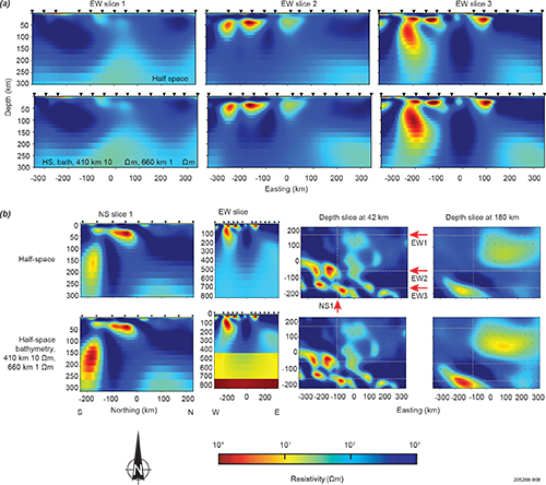
The results are summarised in Table 1. As this survey region is several hundred kilometres from the ocean, bathymetry did not have a large impact on the final model, but this would be more significant in a survey region closer to the ocean. The addition of a conductive layer beneath 410 km served to decrease the overall root mean square fit (RMS – a summation of the difference between the model response and the observed data, weighted by the error), but required significantly longer computational time than the models that do not include this layer. A further addition of another conductive layer beneath 660 km produced another decrease in RMS.
Table 1 Results of four inversions with various starting or prior models
| Model number | Bathymetry | 410 km | 660 km | RMS | Number of iterations |
| 1 | 1.82 | 162 | |||
| 2 | ✓ | 1.98 | 152 | ||
| 3 | ✓ | ✓ | 1.81 | 182 | |
| 4 | ✓ | ✓ | ✓ | 1.71 | 181 |
Notes: The models are numbered for convenience. The overall RMS and the number of iterations for each inversion to converge are provided. The columns refer to models that include bathymetry (row 2), and mantle discontinuities at 410 km (column 3) and 660 km (column 4) due to mineral phase transitions and reduction in resistivity.
It should be stated here that the RMS is not a sufficient method for analysing the fit of the model, it is important that this RMS is relatively evenly distributed amongst each of the MT sites, and across the frequency range of the data. This result and all other modelling results are analysed further in Robertson, Thiel and Meqbel (2020).
Visually, these models have similar appearance, with structures remaining mostly consistent for each of the four models. Some representative cross-sections and depth slices for model 1 (half-space) and model 4 (bathymetry, 410 and 660 km conductive layers) are shown in Figure 2. The models that contain the deep conductivity layers as prior information (models 3 and 4) show very good agreement at crustal depths where the data sensitivity is high, but some of the deeper features are more conductive for these two models.
Figure 2 Comparison of models with prior information included in the starting model. (a) Three east–west cross-sections taken through model 1 (top row) and 4 (bottom row) outlined in Table 1. The cross-sections are located as grey dashed lines in the depth slices below. (b) Left to right: a NS slice; EW slice 3 down to a depth of 800 km to show the deep mantle conductivity; depth slice at 42 km; depth slice at 172 km. Reprinted from Robertson, Thiel and Meqbel (2020, fig. 5 selection) under Creative Commons Licence CC BY 4.0.
Resistivity of the starting model
As previously explained, a starting model is a required input, and here we test the resistivity value of that starting model. For each of these tests, bathymetry (fixed parameter) and a rough representation of underlying ocean sediments (free parameter) were included. The resistivity values tested were 3, 10, 31, 100, 312, 1,000 Ωm (evenly spaced on log scale). In addition, a further value of 69 Ωm was tested representing the average of the apparent resistivity of the data across all periods and all sites.
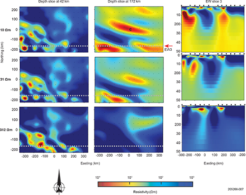
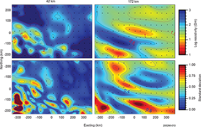
Results from the 10, 31 and 312 Ωm model are shown in Figure 3. These are three of the best-fit models as can be seen in Table 2. They show large variation in the magnitude of the resistivity anomaly. The resistivity and geometry of resistivity structures are visually quite similar for crustal depths, but there is greater difference at mantle depths as can be seen in the standard deviation of the models at 172 km (Fig. 4). Resistivity models are often interpreted qualitatively; the results show that at crustal depths where the data is most sensitive the models show good agreement in mapping structures. At greater depths, however, the changes between models are more pronounced, with a major conductive feature labelled C on the 10 Ωm model in Figure 3 that is not evident in the 312 Ωm model. This could have large consequences for quantitative (and even qualitative) interpretations of these features, with resistivities varying more than an order of magnitude in some parts between models. Thus it is important to understand the model space, and the range of models that can fit the data, and find the model most representative of the data and of the geology. Petrological constraints ideally should be used to help constrain the limits of the resistivity.
Table 2 Overall RMS per starting model
| Starting resistivity (Ωm) | Overall RMS |
| 3.1 | 1.76 |
| 10 | 1.66 |
| 31 | 1.75 |
| 69 | 1.84 |
| 100 | 1.98 |
| 312 | 1.94 |
| 1,000 | 2.06 |
Figure 4 Average and standard deviation of ModEM inversions with prior resistivities of 10, 31.6, 69, 100, 316 and 1000 Ωm. Black triangles are locations of MT sites. A standard deviation of 0.2 at a certain point in the model means that 68% of the data lie within 0.2 log resistivity of the average value of that cell (averaged across all starting models). For example, average value at a point = 100 Ωm (or 2log Ωm), standard deviation = 0.2log Ωm, and then 68% of values lie within ± 0.2log Ωm or between 1.8 and 2.2log Ωm or between 65 and 160 Ωm. The top row shows the average resistivity values (with 0.5 Ωm contours), and the bottom row shows the standard deviation (with 0.2 contours). Reprinted from Robertson, Thiel and Meqbel (2020, fig. 11) under Creative Commons Licence CC BY 4.0.
Covariance testing
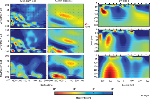
The model covariance is a parameter that controls the inversion codes tendency toward fitting the data, or providing a smooth model. For ModEM3DMT, a high covariance provides a much smoother model, but tends to decrease the data fit, which can be seen in the RMS in Table 3.
As can be seen in Figure 5, adjusting the covariance has a large influence on the final model. The models with a small covariance (0.1) and a large covariance (0.75) have the highest RMS. Further investigation into which is the best model is provided in Robertson, Thiel and Meqbel (2020), but we chose 0.4 as the preferred covariance for this model. It shows a suitable level of detail expected for our survey design, no structural artefacts at the near surface due to lack of sensitivity in between the large site spacing, and a good overall RMS (albeit 14% larger than the lowest RMS of 1.53 for the 0.2 model), that is reasonably well distributed across the full period range of the modelled data.
Table 3 Overall RMS and number of iterations for convergence for selected models
| Covariance* | RMS | Number of iterations |
| 0.1 | 2.17 | 137 |
| 0.2 | 1.53 | 196 |
| 0.3 | 1.6 | 192 |
| 0.4 | 1.75 | 147 |
| 0.5 | 1.97 | 162 |
| 0.75 | 3.86 | 184 |
* The larger the number, the larger the volume over which the smoothing of the model occurs.
Figure 5 Depth slices and cross-section showing models with model covariances of 0.2, 0.4 and 0.75. The test highlights the bias of high model covariance of 0.75 to produce exceedingly strong conductors in the deep mantle. Reprinted from Robertson, Thiel and Meqbel (2020, figs 12 and 13 selection) under Creative Commons Licence CC BY 4.0.
Conclusion
While vast improvements have been made in recent years, 3D inversion of MT datasets is still computationally expensive. As a result, it can be difficult to explore the impact of varying modelling parameters on the final 3D resistivity model.
Our detailed investigation determined the effects of varying modelling parameters using the ModEM3DMT inversion code on a subset of the AusLAMP dataset in northeast South Australia.
The impact of incrementally including prior information to the starting or prior model (bathymetry), then increased conductivity beneath 410 km (10 Ωm), and finally further increased conductivity (1 Ωm) beneath 660 km were tested. The appearance of the final model did not vary too greatly, although the deeper mantle features near the lithosphere–asthenosphere boundary became more conductive for models that included the enhanced conductivity at depth. The ocean is expected to have a bigger impact for a survey region closer to the ocean.
The second test was to vary the starting resistivity (the model was a half-space plus ocean fixed to 0.3 Ωm). Resistivity values of 3, 10, 31, 69, 100, 310 and 1,000 Ωm were tested. Varying the starting resistivity was found to have a large effect on the model, with a more conductive starting model leading to a more conductive final model and vice versa. This test highlights the importance of completing many inversions for a given dataset. We used the average and standard deviation of the final models from the three models that best represented the data and plotted these values at two depths within the model (Fig. 4). This information is useful to explore the model space and understand whether the geometry or magnitude of the resistivity (or both) are constrained by the data.
The last test presented here was varying the model covariance, where a larger covariance produces a smoother model, and a smaller covariance produces a rougher model and a better fit to the data. It is imperative to test a range of model covariances that finds an optimal fit to the data without introducing near-surface ‘speckled’ features. We also found that a larger covariance introduced deep mantle conductors not present with lower covariance, and warrants further investigation.
Despite the difficulties in the practicalities of 3D inversion (access to high-performance computational facilities, queue times to run models, and the time and/or cost associated with these models), these results highlight that it is still critical to test parameters controlling the model space. We show the critical parameters for this dataset to be the starting resistivity of the model and the model covariance. This work presents a guide to inverting MT array data, which is set to become more commonplace with the expansion of surveys such as AusLAMP array and infill MT surveys.
Acknowledgements
All inversions were performed using Raijin from the National Computational Infrastructure in Canberra, Australia, provided by the Australian Government under the National Computational Merit Allocation Scheme. Data was collected by Philippa Mawby, Geoffrey Axford and Bruce Goleby. The MT instruments used were from the AuScope instrumentation pool. Naser Meqbel developed the software 3D grid that was used for generating modelling inputs and viewing some outputs. Most plots were produced using the open-source MT software MTpy (Krieger and Peacock 2014; Kirkby et al. 2019). We thank the authors of ModEM3DMT for making their code accessible.
References
Egbert GD and Kelbert A 2012. Computational recipes for electromagnetic inverse problems. Geophysical Journal International 189(1):251–267.
Heinson G, Didana Y, Soeffky P, Thiel S and Wise T 2018. The crustal geophysical signature of a world-class magmatic mineral system. Scientific Reports 8(1). https://doi.org/10.1038/s41598-018-29016-2 (Open access)
Kelbert A, Meqbel N, Egbert GD and Tandon K 2014. ModEM: a modular system for inversion of electromagnetic geophysical data. Computers and Geosciences 66:40–53.
Kirkby A, Zhang F, Peacock J, Hassan R and Duan J 2019. The MTPy software package for magnetotelluric data analysis and visualisation. Journal of Open Source Software 4:1358.
Krieger L and Peacock J 2014. MTpy: a Python toolbox for magnetotellurics. Computers and Geosciences 72:167–175.
Robertson K, Heinson G and Thiel S 2016. Lithospheric reworking at the Proterozoic–Phanerozoic transition of Australia imaged using AusLAMP magnetotelluric data. Earth and Planetary Science Letters 452:27–35.
Robertson K, Thiel S and Meqbel N 2020. Quality over quantity: on workflow and model space exploration of 3D inversion of MT data. Earth, Planets and Space 72, 2. https://doi.org/10.1186/s40623-019-1125-4 (Open access)
Selway KM, Hand M, Payne JL, Heinson GS and Reid A 2011. Magnetotelluric constraints on the tectonic setting of Grenville-aged orogenesis in central Australia. Journal of the Geological Society 168(1):251–264.
Thiel S and Heinson G 2010. Crustal imaging of a mobile belt using magnetotellurics: an example of the Fowler Domain in South Australia. Journal of Geophysical Research: Solid Earth 115(6):1–18. https://doi.org/10.1029/2009JB006698 (Free access)
Thiel S and Heinson G 2013. Electrical conductors in Archean mantle–result of plume interaction? Geophysical Research Letters 40(12):2947–2952. https://doi.org/10.1002/grl.50486 (Free access)
Thiel S, Heinson G and White A 2005. Tectonic evolution of the southern Gawler Craton, South Australia, from electromagnetic sounding. Australian Journal of Earth Sciences 52(6):887–896.
Thiel S, Soeffky P, Krieger L, Regenauer-Lieb K, Peacock J and Heinson G 2016. Conductivity response to intraplate deformation: evidence for metamorphic devolatilization and crustal-scale fluid focusing. Geophysical Research Letters 43(21):11,236–11,244. https://doi.org/10.1002/2016GL071351 (Free access)
Wise T and Thiel S 2019. Proterozoic tectonothermal processes imaged with magnetotellurics and seismic reflection in southern Australia. Geoscience Frontiers. https://doi.org/10.1016/j.gsf.2019.09.006 (Open access)


