
Lei Huang1, Sandeep Santhosh Kumar1, Wei Ming Ong1, Natalia Pandos1, Melissa Ryan1, Stephan Thiel2, John Boland1, Peter Pudney1 and Lesley Ward1
1 STEM, University of South Australia
2 Geological Survey of South Australia, Department for Energy and Mining
Download this article as a PDF (2.6 MB); cite as MESA Journal 94, pages 41–47
Published June 2021
Introduction
The Mathematics Clinic at the University of South Australia runs a year-long sponsored research project for teams of students in their final year of study in the Bachelor of Mathematics. In 2020 the Department for Energy and Mining partnered with the university, providing the Olympic Domain mineral deposits project.

Figure 1 Location of the study area, Olympic Domain mineral deposits project.
The main aim of the project was to analyse multiple types of geoscientific data to examine relationships between them and mineral deposit locations within the Olympic Domain across a study area of 100 x 100 km near Olympic Dam (Fig 1). Scientific and quantitative method was used to analyse physical properties of the cover and basement rocks as well as the predictive potential of these data to narrow the search space for mineral deposits, in particular copper occurrences. Geophysical data available included:
- gridded topography data, showing the elevation across the study area
- gridded gravity data, showing changes in the gravity field at the surface due to changes in rock density below the surface
- gridded magnetic data, showing changes in the magnetic susceptibility of the rocks near the surface
- gridded airborne electromagnetic data
- gridded 3D resistivity model derived from over 330 broadband magnetotelluric stations
- gridded radiometric data, showing the variation in uranium, thorium and potassium concentration near the surface
- drill core locations and mineral prospect locations.
For our study area, we concluded that the key datasets for predicting likely deposit locations are a combination of raw and derived data, namely magnetic intensity, 2 versions of the slope of low pass filtered (LPF) gravity with different cutoff frequencies, and high pass filtered (HPF) gravity. We completed the project by using a logistic regression model to predict copper deposit locations from the data. This article includes a map of likely copper deposit locations (Fig 7) and details on how it was generated.
Derived data
Early on in the project we decided to extend the number of data layers to include derived data computed from the original datasets outlined above. The derived data layers emphasise specific features of the data. The 2 types of derived data we considered were gradients and frequency filtered datasets. Gradients indicate how much a value changes in a particular direction. Slope is the magnitude of the maximum gradient at a given location. Frequency filtration is the process of isolating specific frequency components of a dataset. Filtering enables separation of small-scale and large-scale spatial features.
Using logistic regression, we found that slopes of the low pass filtered datasets are useful in determining the locations of copper deposits. The low pass filtered datasets contain the long wavelength patterns of the datasets (a few to tens of kilometres in our example), which correspond to deeper features. The slope of a low pass filtered dataset is the slope of the larger features. High pass filtered datasets contain the small-scale and short-wavelength peaks in the datasets – e.g. a gravity high associated with an iron oxide – copper–gold deposit.
Gradients of spatial data
Gradients help us understand the peaks and troughs within the datasets. Geographical features such as faults will often be indicated by large slopes in the data.
The slope of gridded data can be estimated using the neighbourhood slope algorithm (Dunn and Hickey 1998). This numerical method estimates the northwards and eastwards gradients at a point and the maximum rate of change at that point with respect to its neighbours (Horn 1981). This is repeated for each point in the dataset. We used the terrain function in the software package R to calculate slopes. Figure 2 illustrates the result of the computation for the magnetic intensity dataset. The slope quantifies the rate of change of magnetic intensity values with distance in the region.

Figure 2 Magnetic intensity and its slope.
Frequency filtered data
We used spatial frequencies measured per unit distance. For instance, the low pass filter with cutoff frequency 0.05/km removes features with spatial frequencies greater than 0.05/km. This has the effect of removing features which have a spatial wavelength of under 20 km.
A low pass filtered dataset brings out the larger or long-wavelength features of the data, which often correspond to deeper subsurface structures. The high pass filtered data contains more rapid changes in the data; these are often caused by structures closer to the surface.
Our filtration process used a 2D discrete Fourier transform, which transformed the data into the frequency domain. Unwanted frequencies were removed and the filtered data was obtained by applying an inverse 2D discrete Fourier transform. We created 2 R functions, filterglp and filterghp, which apply Gaussian filtering to the data. An example for the magnetic intensity is shown in Figure 3.

Figure 3 Magnetic intensity, with Gaussian low pass and high pass filtered versions.
Logistic regression
We used a multivariable logistic regression model to determine the probability of finding a copper deposit at a particular location using the geophysical datasets provided by the department and our derived data. How logistic regression works is demonstrated through examples given below (see 'Applying logistic regression'). Akaike information criterion (AIC) backward elimination was used to select 11 significant parameters out of 19 (see 'Using the AIC method') to fit a logistic regression model. The model was further simplified through trial and error, narrowing down the number of parameters to 4 (see 'Further simplification of the model'). The predictive capability of the model was checked by examining how well it fitted the data (see 'How good are the predictions?'). Using the 4-parameter model we created a copper deposit prediction map of the whole study region (Fig 7).
Regression analysis is used to determine the relationship between 2 or more variables. Logistic regression is used when the desired prediction outcome is binary. For our application, a location is either a deposit or a non-deposit. We defined non-deposits as drillhole locations more than 5 km away from a known copper deposit. Geophysical data was used to predict the probability of a location having a copper deposit.
The general concept of logistic regression is to fit a logistic curve to the data. A logistic curve has the form
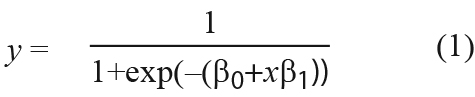
where y is the binary variable to be predicted from variable x, and β0 and β1 are constants (Brownlee 2019).
For our model, y is the probability of a location containing a copper deposit and x is a geophysical parameter.
The values of different geophysical parameters have different ranges. Before applying logistic regression, we standardised the parameter values by calculating z- scores
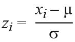
where xi is an original value from a parameter, µ is the mean value for that parameter, and σ is the standard deviation of values for that parameter. Standardising the parameter values allowed us to compare the coefficients, β0 and β1, of different logistic regression analyses.
Applying logistic regression
Application of the logistic regression method is illustrated herein on magnetic intensity and uranium concentration data respectively.
Figure 4 shows the fitted logistic regression curve from the magnetic intensity data. The horizontal axis shows standardised magnetic intensity values. The data points at the top of the plot with y = 1 correspond to deposit locations, and the points at the bottom correspond to non-deposit locations. Logistic regression analysis fits a logistic curve to these points. The y value from the curve gives the probability of finding a deposit based on the x-axis value of standardised magnetic intensity.

Figure 4 Logistic regression of magnetic intensity.
Table 1 summarises the regression analysis results. The constants β0 and β1 are from equation (1). The p-value of β1 indicates that the coefficient is statistically significant. For magnetic intensity the p-value of β1 is very small, so β1 is a meaningful coefficient. The value of β1 is positive, which indicates that the probability of a copper deposit increases with magnetic intensity. The AIC score is used to compare different statistical models. The smaller the AIC score, the better the model. This score is explained in more detail below ('Using the AIC method').
Table 1 Summary of logistic regression of magnetic intensity
| β0 | β1 | p-value of β1 | AIC |
|---|---|---|---|
| –2.7615 | 0.5438 | 1.83 x 10⁻⁷ | 324.82 |
Figure 5 shows the logistic curve fitted to the uranium concentration data. The logistic regression curve is almost a straight line – every value of standardised uranium concentration corresponds to a low probability of a deposit. By examining the regression analysis summary from Table 2, we see that the p-value of coefficient β1 is greater than 0.05 which indicates β1 is not a meaningful coefficient. The associated AIC score is also larger than that for the model with magnetic intensity, meaning that magnetic intensity produces a better regression model. We conclude that uranium concentration is not a good predictor of copper deposits.

Figure 5 Logistic regression of uranium concentration.
Table 2 Summary of logistic regression of uranium concentration
| β0 | β1 | p-value of β1 | AIC |
|---|---|---|---|
| –2.39661 | –0.06902 | 0.617 | 361.19 |
In a similar manner, we can create a multivariable logistic regression model that simultaneously takes into account more than one geophysical parameter.
Using the AIC method to determine relevant geophysical parameters
To create a logistic regression model that considers many different geophysical parameters we needed to determine which parameters are important.
The AIC quantifies the relative quality of statistical models enabling comparison of logistic regression models made using different parameters. A better model will have a smaller AIC score. The score improves as the number of parameters in the model is reduced, and as the loglikelihood – a measure of how well the model fits the data – increases (Glen 2015).
AIC backward elimination is an automated method of finding appropriate predictor parameters for a multivariable regression model. The process starts by considering a model with all of the parameters. It then removes the parameter that has the least contribution to the AIC score. The process of removing parameters is repeated until the model’s AIC score is minimised (Tripathi 2019).
We performed AIC backward elimination on an initial model that included 19 parameters for which the data covered the entire region, so that we could use all of the known deposit and non-deposit locations. The backward elimination was done using the R function stepAIC from the package MASS.
The parameters in order of removal were:
- dose rate
- magnetics
- slope of gravity
- gravity LPF, 0.1/km
- uranium concentration
- topography
- potassium concentration
- thorium concentration.
The 11 parameters remaining were:
- slope of gravity LPF, 0.05/km
- slope of gravity LPF, 0.1/km
- magnetics HPF, 0.05/km
- slope of magnetics LPF, 0.05/km
- slope of magnetics LPF, 0.1/km
- magnetics LPF, 0.05/km
- magnetics LPF, 0.1/km
- slope of magnetics
- gravity
- gravity LPF, 0.05/km
- gravity HPF, 0.05/km.
Further simplification of the model by trial and error
Through trial and error we found 4 parameters that maintain significant coefficients when combined together to make a logistic regression model:
- magnetic intensity
- HPF residual gravity, 0.05/kmcutoff frequency
- slope of LPF residual gravity, 0.1/km cutoff frequency
- slope of LPF residual gravity, 0.05/km cutoff frequency.
We initially assumed that drillhole locations that are more than 5 km away from a known copper deposit are non-deposit locations. We also made logistic regression models by fitting data with non-deposit locations defined as drillhole locations that are over 0.5 km and 10 km away from known copper deposit locations. Our 4 chosen parameters maintained significant coefficients for each of these different models. Even though some of the parameters used in this model were eliminated by AIC backward elimination, the AIC score of this model is better than the result using 11 parameters. Our final model is summarised in Table 3.
Table 3 Parameters used in final logistic regression model to predict copper deposit locations
| Parameter | Coefficient | Standard error | z value | P[> |z|] |
|---|---|---|---|---|
| (Intercept) | –3.5647 | 0.2948 | –12.093 | < 2 x 10-16 |
| Magnetics | 0.9032 | 0.1701 | 5.309 | 1.10 x 10-07 |
| Slope of gravity LPF 0.1/km | –1.2518 | 0.3262 | –3.837 | 1.24 x 10-04 |
| Slope of gravity LPF 0.05/km | 1.5620 | 0.2907 | 5.373 | 7.73 x 10-08 |
| Gravity HPF 0.05/km | 0.5873 | 0.1327 | 4.425 | 9.66 x 10-06 |
Figure 6 shows maps of the 4 parameters used in the final logistic regression model. The high pass filtered version of gravity contains the small-scale peaks of the residual gravity dataset. The slope of low pass filtered versions of gravity contains the slope of the larger features in the dataset. Two versions of the slope of low pass filtered residual gravity are used by the model, with cutoff frequencies of 0.1/km and 0.05/km. The 2 versions look at features that are larger than 2 different sizes. It is unclear why they are both significant in the model, especially considering that one of the coefficients is negative. Nonetheless, they do have significant coefficients, and thus contribute to the predictive capability of the model. It is interesting to note a statistically significant relationship between large-scale features of the residual gravity dataset and deposits.

Figure 6 Maps of the 4 parameters used by the logistic regression model. The blue triangles are known deposits and the black circles are drillhole locations.
How good are the predictions?
Table 4 shows results from the simplified model when we applied it to the deposit and non-deposit locations used to construct the model.
Table 4 Performance of predictions by the logistic regression model
| P[deposit] | ≥0.00 | ≥0.25 | ≥0.5 | ≥0.75 |
|---|---|---|---|---|
| Number of copper deposit locations | 52 | 29 | 19 | 12 |
| Number of non-deposit locations | 479 | 24 | 7 | 2 |
| Percentage of deposit locations | 10 | 55 | 73 | 85 |
If we consider the locations where the probability of a copper deposit as predicted by the model is greater than 0.75, we see that 12 of these locations are copper deposits and 2 are non-deposits. Hence, if we pick a location randomly out of this set of locations, there is an 85% chance that the location is a deposit. This is much greater than the chance of getting a copper deposit if we pick a location randomly out of all the locations (10%).
Prediction map
The simplified model was used to predict the presence of deposits in the study area (Fig 7). The dark red regions indicate likely copper deposits. Some of these locations do not have drillholes near them and may be worth exploring.

Figure 7 Predicted copper deposit locations in the 100 x 100 km study area using the simplified 4-parameter model. Dark red indicates a high probability of copper deposits. The blue triangles are known deposits and the black circles are drillhole locations.
Summary
Logistic regression provided the best results compared to clustering and correlation techniques we investigated. It allowed us to determine the prediction capability of different geophysical parameters. Using AIC backward elimination, we were able to narrow down the number of parameters from 19 to 11. Further simplification of the model reduced the number of parameters to 4, namely magnetic intensity, high pass filtered residual gravity with a cutoff frequency of 0.05/km and 2 versions of the slope of low pass filtered residual gravity with cutoff frequencies of 0.1/km and 0.05/km. A review of our predictions showed the simplified 4-parameter model significantly increases the chance of finding a copper deposit. Nonetheless, these are not necessarily the absolute best parameters.
Our predictive model uses the slope of the low pass filtered residual gravity; these are the slopes of the larger, deeper features of the gravity dataset. This shows that the larger features of the residual gravity dataset are informative in determining the presence of copper deposits. It suggests that for direct targeting of deposits, the regional trends in the geology highlighting the edges of lithological basement units is equally important as the gravity highs associated with the deposits themselves.
Using our final simplified model, we made a map predicting the location of copper deposits in the Olympic Domain region (Fig 7).
Conclusion
Using logistic regression on geophysical datasets and derived datasets to predict copper deposit locations we determined 4 important datasets that together indicate prospective copper deposit locations – magnetic intensity, 2 versions of the slope of low pass filtered residual gravity with different cutoff frequencies, and high pass filtered residual gravity. These 4 parameters were used to fit a logistic regression model to predict the probability of copper deposit locations in the form of a prediction map. Our simplified 4-parameter model significantly increases the chance of finding a copper deposit.
Future work that could add to the results obtained so far includes:
- Investigating if there are other parameters important in locating copper deposits and introducing these into the model to potentially improve the prediction accuracy.
- Applying the current model to other regions, or to an expansion of our 100 x 100 km study area, to see whether similar results are obtained.
References
Dunn M and Hickey R 1998. The effect of slope algorithms on slope estimates within a GIS. Cartography 27:9–15. doi:10.1080/00690805.1998.9714086.
Horn B 1981. Hill shading and the reflectance map. Proceedings of the IEEE 69: 14–47. doi:10.1109/PROC.1981.11918.
Tripathi A 2019. What is stepAIC in R? Medium website, accessed 23 October 2020.